The material is based on my workshop at Berkeley - Machine learning with scikit-learn. I convert it here so that there will be more explanation. Note that, the code is written using Python 3.6. It is better to read the slides I have first, which you can find it here. You can find the notebook on Qingkai's Github.
Scikit-learn Basics
In the next few weeks, we will introduce scikit-learn, a popular package containing a collection of tools for machine learning written in Python. See more at http://scikit-learn.org. It has many existing algorithms that implemented and tested by many volunteers, therefore, before you decide to write some algorithms by yourself, check if it is already there.
The first thing when you build a working machine learning algorithm, you need data. You can always start with your own data from specific problems, but you can also first build a prototype using existing data that already included in scikit-learn.
Loading an example dataset
Let's start by loading some pre-existing datasets in the scikit-learn, which comes with a few standard datasets. For example, the iris and digits datasets for classification and the boston house prices dataset for regression. Using these existing datasets, we can easily test the algorithms that we are interested in.
A dataset is a dictionary-like object that holds all the data and some metadata about the data. This data is stored in the .data member, which is a n_samples, n_features array. In the case of supervised problem, one or more response variables are stored in the .target member. More details on the different datasets can be found in the dedicated section.
Load iris
The iris dataset consists of 50 samples from each of three species of Iris (Iris setosa, Iris virginica and Iris versicolor). Four features were measured from each sample: the length and the width of the sepals and petals, in centimetres.
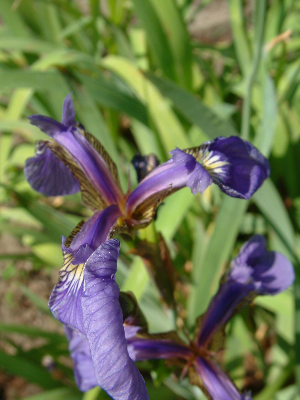 | 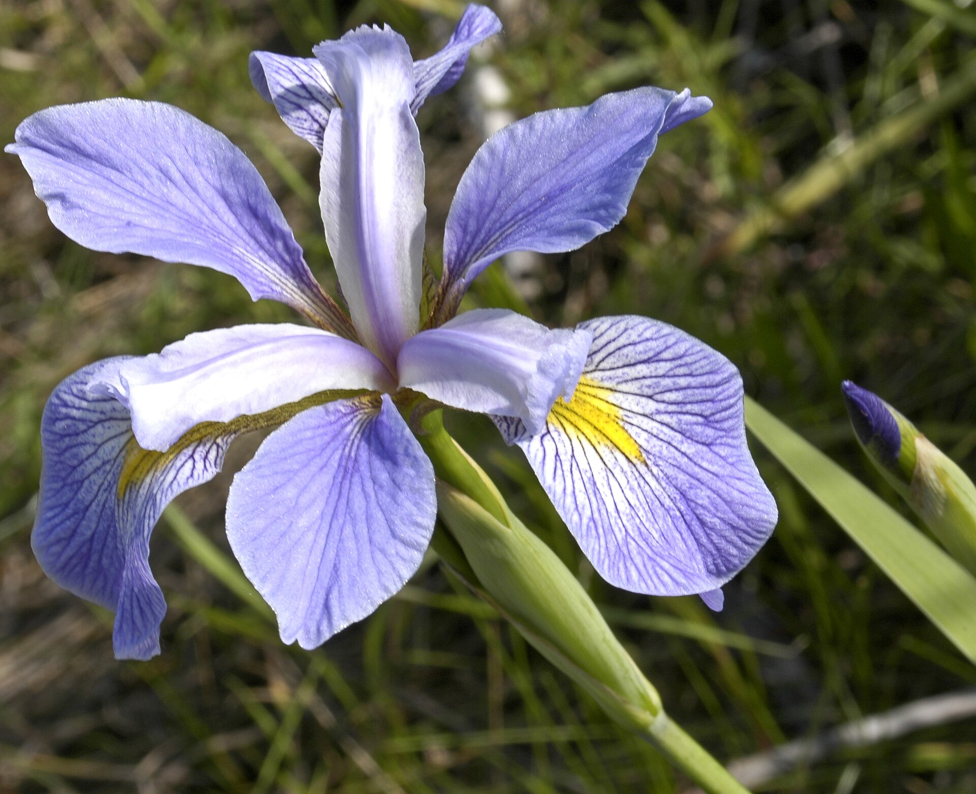 |  |
|---|---|---|
| Iris Setosa | Iris Virginica | Iris Versicolor |
import warnings
warnings.filterwarnings("ignore")

from sklearn import datasets
import matplotlib.pyplot as plt
import numpy as np

plt.style.use('seaborn-poster')
%matplotlib inline
# load the data
iris = datasets.load_iris()
print(iris.keys())dict_keys(['data', 'target', 'target_names', 'DESCR', 'feature_names'])
There are five keys here, and data and target are storing the data and the label we are interested. feature_names and target_names are the corresponding header names. The DESCR has a list of information about this dataset. Let's print out each one of them and have a look.
print(iris.feature_names)
# only print the first 10 samples
print(iris.data[:10])
print('We have %d data samples with %d features'%(iris.data.shape[0], iris.data.shape[1]))
['sepal length (cm)', 'sepal width (cm)', 'petal length (cm)', 'petal width (cm)']
[[ 5.1 3.5 1.4 0.2]
[ 4.9 3. 1.4 0.2]
[ 4.7 3.2 1.3 0.2]
[ 4.6 3.1 1.5 0.2]
[ 5. 3.6 1.4 0.2]
[ 5.4 3.9 1.7 0.4]
[ 4.6 3.4 1.4 0.3]
[ 5. 3.4 1.5 0.2]
[ 4.4 2.9 1.4 0.2]
[ 4.9 3.1 1.5 0.1]]
We have 150 data samples with 4 features
The data is always a 2D array, shape (n_samples, n_features), although the original data may have had a different shape. The following prints out the target names and the representation of the target using 0, 1, 2. Each of them represents a class.
print(iris.target_names)
print(set(iris.target))
['setosa' 'versicolor' 'virginica']
{0, 1, 2}print(iris.DESCR)Iris Plants Database
====================
Notes
-----
Data Set Characteristics:
:Number of Instances: 150 (50 in each of three classes)
:Number of Attributes: 4 numeric, predictive attributes and the class
:Attribute Information:
- sepal length in cm
- sepal width in cm
- petal length in cm
- petal width in cm
- class:
- Iris-Setosa
- Iris-Versicolour
- Iris-Virginica
:Summary Statistics:
============== ==== ==== ======= ===== ====================
Min Max Mean SD Class Correlation
============== ==== ==== ======= ===== ====================
sepal length: 4.3 7.9 5.84 0.83 0.7826
sepal width: 2.0 4.4 3.05 0.43 -0.4194
petal length: 1.0 6.9 3.76 1.76 0.9490 (high!)
petal width: 0.1 2.5 1.20 0.76 0.9565 (high!)
============== ==== ==== ======= ===== ====================
:Missing Attribute Values: None
:Class Distribution: 33.3% for each of 3 classes.
:Creator: R.A. Fisher
:Donor: Michael Marshall (MARSHALL%PLU@io.arc.nasa.gov)
:Date: July, 1988
This is a copy of UCI ML iris datasets.
http://archive.ics.uci.edu/ml/datasets/Iris
The famous Iris database, first used by Sir R.A Fisher
This is perhaps the best known database to be found in the
pattern recognition literature. Fisher's paper is a classic in the field and
is referenced frequently to this day. (See Duda & Hart, for example.) The
data set contains 3 classes of 50 instances each, where each class refers to a
type of iris plant. One class is linearly separable from the other 2; the
latter are NOT linearly separable from each other.
References
----------
- Fisher,R.A. "The use of multiple measurements in taxonomic problems"
Annual Eugenics, 7, Part II, 179-188 (1936); also in "Contributions to
Mathematical Statistics" (John Wiley, NY, 1950).
- Duda,R.O., & Hart,P.E. (1973) Pattern Classification and Scene Analysis.
(Q327.D83) John Wiley & Sons. ISBN 0-471-22361-1. See page 218.
- Dasarathy, B.V. (1980) "Nosing Around the Neighborhood: A New System
Structure and Classification Rule for Recognition in Partially Exposed
Environments". IEEE Transactions on Pattern Analysis and Machine
Intelligence, Vol. PAMI-2, No. 1, 67-71.
- Gates, G.W. (1972) "The Reduced Nearest Neighbor Rule". IEEE Transactions
on Information Theory, May 1972, 431-433.
- See also: 1988 MLC Proceedings, 54-64. Cheeseman et al"s AUTOCLASS II
conceptual clustering system finds 3 classes in the data.
- Many, many more ...Load Digits
This dataset is made up of 1797 8x8 images. Each image, like the ones shown below, is of a hand-written digit. In order to utilize an 8x8 figure like this, we’d have to first transform it into a feature vector with length 64.
digits = datasets.load_digits()
print('We have %d samples'%len(digits.target))
We have 1797 samplesprint(digits.data)
print('The targets are:')
print(digits.target_names)[[ 0. 0. 5. ..., 0. 0. 0.]
[ 0. 0. 0. ..., 10. 0. 0.]
[ 0. 0. 0. ..., 16. 9. 0.]
...,
[ 0. 0. 1. ..., 6. 0. 0.]
[ 0. 0. 2. ..., 12. 0. 0.]
[ 0. 0. 10. ..., 12. 1. 0.]]
The targets are:
[0 1 2 3 4 5 6 7 8 9]
In the digits, each original sample is an image of shape (8, 8) and it is flattened into a 64 dimension vector here.
print(digits.data.shape)(1797, 64)## plot the first 64 samples, and get a sense of the data
fig = plt.figure(figsize = (8,8))
fig.subplots_adjust(left=0, right=1, bottom=0, top=1, hspace=0.05, wspace=0.05)
for i in range(64):
ax = fig.add_subplot(8, 8, i+1, xticks=[], yticks=[])
ax.imshow(digits.images[i],cmap=plt.cm.binary,interpolation='nearest')
ax.text(0, 7, str(digits.target[i]))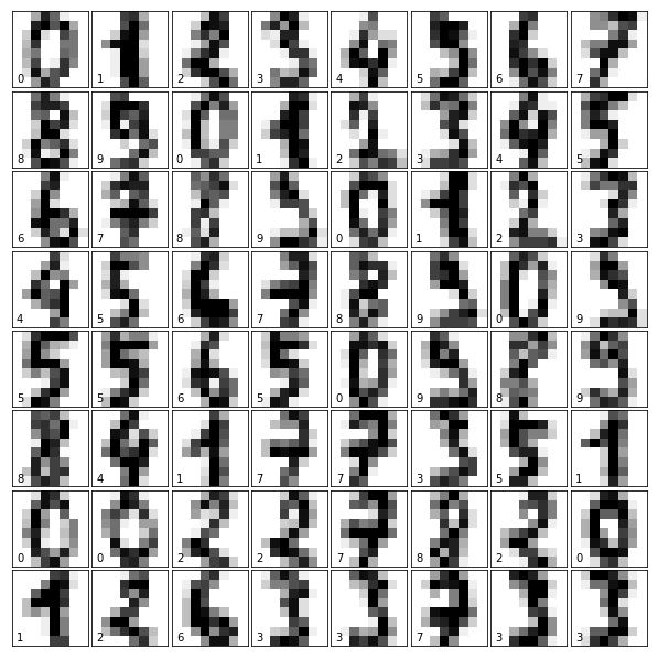
Load Boston Housing Data
The Boston housing dataset reports the median value of owner-occupied homes in various places in the Boston area, together with several variables which might help to explain the variation in median value, such as Crime (CRIM), areas of non-retail business in the town (INDUS), the age of people who own the house (AGE), and there are many other attributes that you can find the details here.
boston = datasets.load_boston()
print(boston.DESCR)
Boston House Prices dataset
===========================
Notes
------
Data Set Characteristics:
:Number of Instances: 506
:Number of Attributes: 13 numeric/categorical predictive
:Median Value (attribute 14) is usually the target
:Attribute Information (in order):
- CRIM per capita crime rate by town
- ZN proportion of residential land zoned for lots over 25,000 sq.ft.
- INDUS proportion of non-retail business acres per town
- CHAS Charles River dummy variable (= 1 if tract bounds river; 0 otherwise)
- NOX nitric oxides concentration (parts per 10 million)
- RM average number of rooms per dwelling
- AGE proportion of owner-occupied units built prior to 1940
- DIS weighted distances to five Boston employment centres
- RAD index of accessibility to radial highways
- TAX full-value property-tax rate per $10,000
- PTRATIO pupil-teacher ratio by town
- B 1000(Bk - 0.63)^2 where Bk is the proportion of blacks by town
- LSTAT % lower status of the population
- MEDV Median value of owner-occupied homes in $1000's
:Missing Attribute Values: None
:Creator: Harrison, D. and Rubinfeld, D.L.
This is a copy of UCI ML housing dataset.
http://archive.ics.uci.edu/ml/datasets/Housing
This dataset was taken from the StatLib library which is maintained at Carnegie Mellon University.
The Boston house-price data of Harrison, D. and Rubinfeld, D.L. 'Hedonic
prices and the demand for clean air', J. Environ. Economics & Management,
vol.5, 81-102, 1978. Used in Belsley, Kuh & Welsch, 'Regression diagnostics
...', Wiley, 1980. N.B. Various transformations are used in the table on
pages 244-261 of the latter.
The Boston house-price data has been used in many machine learning papers that address regression
problems.
**References**
- Belsley, Kuh & Welsch, 'Regression diagnostics: Identifying Influential Data and Sources of Collinearity', Wiley, 1980. 244-261.
- Quinlan,R. (1993). Combining Instance-Based and Model-Based Learning. In Proceedings on the Tenth International Conference of Machine Learning, 236-243, University of Massachusetts, Amherst. Morgan Kaufmann.
- many more! (see http://archive.ics.uci.edu/ml/datasets/Housing)boston.feature_namesarray(['CRIM', 'ZN', 'INDUS', 'CHAS', 'NOX', 'RM', 'AGE', 'DIS', 'RAD',
'TAX', 'PTRATIO', 'B', 'LSTAT'],
dtype='<U7')# let's just plot the average number of rooms per dwelling with the price
plt.figure(figsize = (10,8))
plt.plot(boston.data[:,5], boston.target, 'o')
plt.xlabel('Number of rooms')
plt.ylabel('Price (thousands)')<matplotlib.text.Text at 0x10f4a40f0>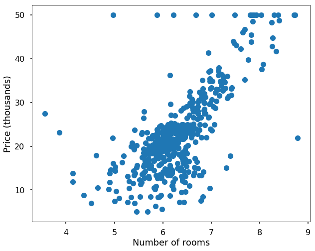
The Scikit-learn Estimator Object
Every algorithm is exposed in scikit-learn via an ''Estimator'' object. For instance a linear regression is implemented as so:
from sklearn.linear_model import LinearRegression
Estimator parameters: All the parameters of an estimator can be set when it is instantiated, and have suitable default values:
# you can check the parameters as
LinearRegression?
# let's change one parameter
model = LinearRegression(normalize=True)
print(model.normalize)Trueprint(model)LinearRegression(copy_X=True, fit_intercept=True, n_jobs=1, normalize=True)
Estimated Model parameters: When data is fit with an estimator, parameters are estimated from the data at hand. All the estimated parameters are attributes of the estimator object ending by an underscore:
Simple regression problem
Let's fit a simple linear regression model to see what is the sklearn API looks like. We use a very simple dataset with 10 samples with added in noise.
x = np.arange(10)
y = 2 * x + 1plt.figure(figsize = (10,8))
plt.plot(x,y,'o')[<matplotlib.lines.Line2D at 0x10fdcacc0>]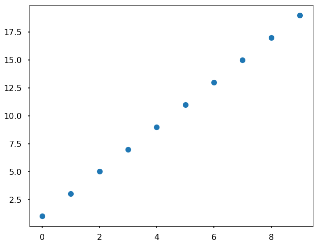
# generate noise between -1 to 1
# this seed is just to make sure your results are the same as mine
np.random.seed(42)
noise = 2 * np.random.rand(10) - 1

# add noise to the data
y_noise = y + noiseplt.figure(figsize = (10,8))
plt.plot(x,y_noise,'o')[<matplotlib.lines.Line2D at 0x10ff89b70>]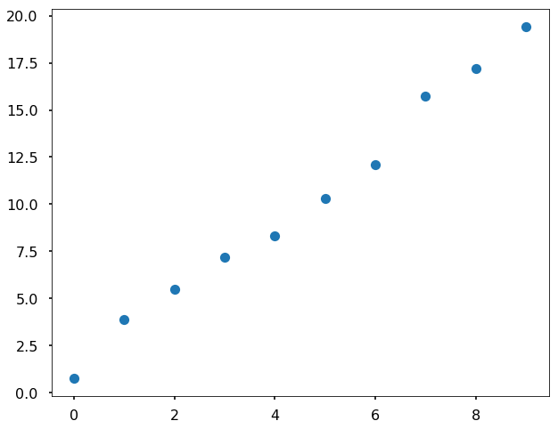
# The input data for sklearn is 2D: (samples == 10 x features == 1)
X = x[:, np.newaxis]
print(X)
print(y_noise)
[[0]
[1]
[2]
[3]
[4]
[5]
[6]
[7]
[8]
[9]]
[ 0.74908024 3.90142861 5.46398788 7.19731697 8.31203728
10.31198904 12.11616722 15.73235229 17.20223002 19.41614516]# model fitting is via the fit function
model.fit(X, y_noise)LinearRegression(copy_X=True, fit_intercept=True, n_jobs=1, normalize=True)# underscore at the end indicates a fit parameter
print(model.coef_)
print(model.intercept_)[ 1.99519708]
1.06188659819# then we can use the fitted model to predict new data
predicted = model.predict(X)plt.figure(figsize = (10,8))
plt.plot(x,y_noise,'o')
plt.plot(x,predicted, label = 'Prediction')
plt.legend()<matplotlib.legend.Legend at 0x11014bb00>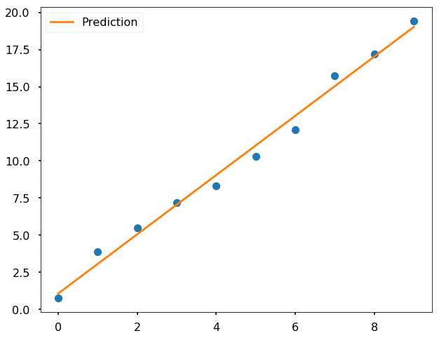
ReplyDeleteIt is really a great work and the way in which u r sharing the knowledge is excellent.Thanks for helping me to understand How it works. Thanks for your informative article
Also Check out the : https://www.credosystemz.com/training-in-chennai/best-data-science-training-in-chennai/
DR EMU WHO HELP PEOPLE IN ANY TYPE OF LOTTERY NUMBERS
DeleteIt is a very hard situation when playing the lottery and never won, or keep winning low fund not up to 100 bucks, i have been a victim of such a tough life, the biggest fund i have ever won was 100 bucks, and i have been playing lottery for almost 12 years now, things suddenly change the moment i came across a secret online, a testimony of a spell caster called dr emu, who help people in any type of lottery numbers, i was not easily convinced, but i decided to give try, now i am a proud lottery winner with the help of dr emu, i won $1,000.0000.00 and i am making this known to every one out there who have been trying all day to win the lottery, believe me this is the only way to win the lottery.
Dr Emu can also help you fix this issues
(1)Ex back.
(2)Herbal cure & Spiritual healing.
(3)You want to be promoted in your office.
(4)Pregnancy spell.
(5)Win a court case.
Contact him on email Emutemple@gmail.com
What's app +2347012841542
Website Https://emutemple.wordpress.com/
Https://web.facebook.com/Emu-Temple-104891335203341
Good Blog
ReplyDeleteThanks For Sharing
Machine learning in Vijayawada
Five weeks ago my boyfriend broke up with me. It all started when i went to summer camp i was trying to contact him but it was not going through. So when I came back from camp I saw him with a young lady kissing in his bed room, I was frustrated and it gave me a sleepless night. I thought he will come back to apologies but he didn't come for almost three week i was really hurt but i thank Dr.Azuka for all he did i met Dr.Azuka during my search at the internet i decided to contact him on his email dr.azukasolutionhome@gmail.com he brought my boyfriend back to me just within 48 hours i am really happy. What’s app contact : +44 7520 636249
ReplyDeletebest post.
ReplyDeleteMachine Learning Course in Hyderabad
Machine Learning Training in Hyderabad