I am going to teach a workshop on Artificial Neural Networks at Berkeley D-Lab. Therefore, this week, I will just show my slides I created. There are many slides I converted from the blogs I wrote in the past few weeks, but it also contains some more interesting stuff, check it out! Also, you can download all the related materials (notebooks) on Qingkai's Github. Happy Thanks Giving!
Friday, November 25, 2016
Sunday, November 20, 2016
Machine learning 6 - Artificial Neural Networks - part 4- sklearn MLP classification example
We discussed the basics of Artificial Neural Network (or Multi-Layer Perceptron) in the last few weeks. Now you can implement a simple version of ANN by yourself, but there are already many packages online that you can use it with more flexible settings. This week, we will give an example of using MLP from the awesome scikit-learn. You can also check their website about the introduction of the ANN.
We will work on the famous Handwritten Digits Data Sets, and classify the digits using MLP. Recognizing handwritten digits is vastly used everywhere these days, for example, when you deposit a check at ATM, an algorithm similar to what we will cover here to recognize the number you wrote.
We will show the basic working flow of using the MLP classifier in sklearn, and hope you can use this as an initial start in your research. Let's start now!
# import all the needed module
import itertools
from sklearn.datasets import load_digits
import matplotlib.pyplot as plt
from sklearn.model_selection import train_test_split
from sklearn.neural_network import MLPClassifier
from sklearn.preprocessing import StandardScaler
from sklearn.metrics import classification_report,confusion_matrix
import numpy as np
plt.style.use('seaborn-poster')
%matplotlib inline
Load and visualize data
Let's load the Handwritten Digits Data Set from sklearn. The data set contains images of handwritten digits: 10 classes where each class refers to a digit from 0 to 9. In sklearn, it includes a subset of the handwritten data for quick testing purposes, therefore, we will use this subset as an example. Load the data first:
# load data
digits = load_digits()
print('We have %d samples'%len(digits.target))
We have 1797 samples
The data that we are interested in is made of 8x8 images of digits, and we will plot the first 64 samples below, and get a sense what we will work with. Each image shows the handwritten digit and the correct digit on the left bottom corner.
## plot the first 64 samples, and get a sense of the data
fig = plt.figure(figsize = (8,8))
fig.subplots_adjust(left=0, right=1, bottom=0, top=1, hspace=0.05, wspace=0.05)
for i in range(64):
    ax = fig.add_subplot(8, 8, i+1, xticks=[], yticks=[])
    ax.imshow(digits.images[i],cmap=plt.cm.binary,interpolation='nearest')
    ax.text(0, 7, str(digits.target[i]))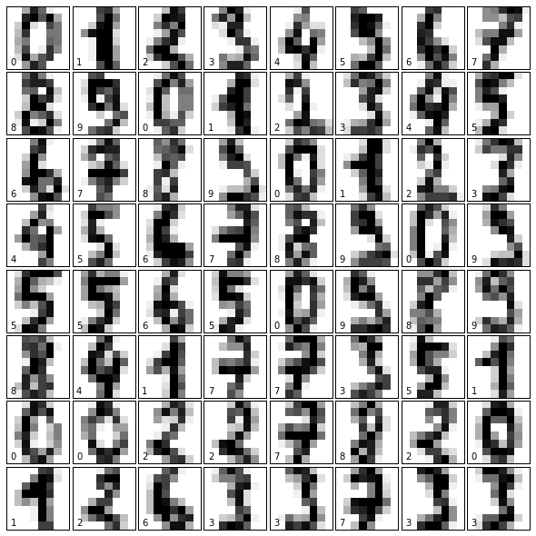
Train an ANN classifier
We will split the whole data into 80% training data and 20% test data. We then will build an ANN model using the default parameter setting, and train it using the training data.
# split data to training and testing data
X_train, X_test, y_train, y_test = train_test_split(digits.data, digits.target, test_size=0.2, random_state=16)
print('Number of samples in training set: %d, number of samples in test set: %d'%(len(y_train), len(y_test)))
Number of samples in training set: 1437, number of samples in test set: 360
The next step is doing pre-processing of the data. In simple words, pre-processing refers to the transformations applied to your data before feeding it to the algorithm. Usually, the pre-processing can transform the data to the range of 0 to 1, or zero mean and unit variance, and so on. Here, we will use the StandardScaler in sklearn to scale the data to zero mean and unit variance.
scaler = StandardScaler()
# Fit only to the training data
scaler.fit(X_train)

# Now apply the transformations to the data:
X_train_scaled = scaler.transform(X_train)
X_test_scaled = scaler.transform(X_test)
The following code block is to train the MLP classifier. We will mostly use the default setting, and you can find more details information of the options here.
# Initialize ANN classifier
mlp = MLPClassifier(hidden_layer_sizes=(30,30,30), activation='logistic', max_iter = 1000)

# Train the classifier with the traning data
mlp.fit(X_train_scaled,y_train)
MLPClassifier(activation='logistic', alpha=0.0001, batch_size='auto',
beta_1=0.9, beta_2=0.999, early_stopping=False, epsilon=1e-08,
hidden_layer_sizes=(30, 30, 30), learning_rate='constant',
learning_rate_init=0.001, max_iter=1000, momentum=0.9,
nesterovs_momentum=True, power_t=0.5, random_state=None,
shuffle=True, solver='adam', tol=0.0001, validation_fraction=0.1,
verbose=False, warm_start=False)
I will explain the options usually you need change or know briefly here:
* activation - this is to define different activation functions.
* alpha - this parameter controls the regularization which help avoiding overfitting.
* solver - the option to choose different algorithm for weight optimization. * batchsize - size of minibatches for stochastic optimizers. This is the option that will decide how much samples will be used in online learning.
* learningrate - option to use different learning rate for weight updates. You can use constant learning rate, or changing the learning rate with progress.
* max_iter - maximum number of iterations. This will decide when to stop the solver, either the solver converges (determined by 'tol') or this maximum number of iterations.
* tol - tolerance for the optimization.
* momentum - momentum for gradient descent update. This will try to avoid trap the local minimum.
Test ANN classifier and evaluate
After we trained the ANN classifier, we will test the performance of the classifier using the test data. To evaluate the results, we will plot the confusion matrix.
def plot_confusion_matrix(cm, classes,
                          normalize=False,
                          title='Confusion matrix',
                          cmap=plt.cm.Blues):
    """
    This function prints and plots the confusion matrix.
    Normalization can be applied by setting `normalize=True`.
    """
    fig = plt.figure(figsize=(8, 8))
    plt.imshow(cm, interpolation='nearest', cmap=cmap)
    plt.title(title)
    plt.colorbar()
    tick_marks = np.arange(len(classes))
    plt.xticks(tick_marks, classes, rotation=45)
    plt.yticks(tick_marks, classes)

    if normalize:
        cm = cm.astype('float') / cm.sum(axis=1)[:, np.newaxis]

    thresh = cm.max() / 2.
    for i, j in itertools.product(range(cm.shape[0]), range(cm.shape[1])):
        plt.text(j, i, cm[i, j],
                 horizontalalignment="center",
                 color="white" if cm[i, j] > thresh else "black")

    plt.tight_layout()
    plt.ylabel('True label')
    plt.xlabel('Predicted label')
    plt.show()
# predict results from the test data
predicted = mlp.predict(X_test_scaled)
# plot the confusion matrix
cm = confusion_matrix(y_test,predicted)
plot_confusion_matrix(cm, classes=digits.target_names,
title='Confusion matrix, without normalization')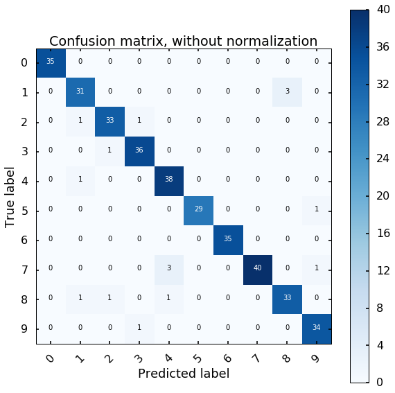
The x axis is the predicted digit from the MLP model, and the y axis is the true digit. The diagonal represents the correct results, we can see most of the digits we can estimate correctly. If we look at the first row, the off-diagonal number represents how many digits we estimate wrong for the digit 0, if there is 1 at the 6th column, this means that we classify one 0 digit to 5.
Visualize the test results
Let's visualize the first 64 digits in the test data. The green or the red digits at the left bottom corner are our estimation from the MLP model. Green means we correctly classified the data, and red indicates the model did wrong.
expected = y_test
fig = plt.figure(figsize=(8, 8))  # figure size in inches
fig.subplots_adjust(left=0, right=1, bottom=0, top=1, hspace=0.05, wspace=0.05)

# plot the digits: each image is 8x8 pixels
for i in range(64):
    ax = fig.add_subplot(8, 8, i + 1, xticks=[], yticks=[])
    ax.imshow(X_test.reshape(-1, 8, 8)[i], cmap=plt.cm.binary, interpolation='nearest')

    # label the image with the target value
    if predicted[i] == expected[i]:
        ax.text(0, 7, str(predicted[i]), color='green')
    else:
        ax.text(0, 7, str(predicted[i]), color='red')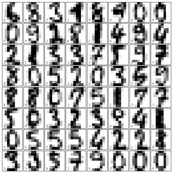
Saturday, November 12, 2016
Machine learning 5 - Artificial Neural Networks - part 3- Step by step implement Muti-Layer Perceptron (MLP)
In the previous blog, we implemented a simple Perceptron algorithm and explained all the important part of it. We concluded with a statement that, Perceptron has its own limitation which actually causing the winter of ANN in the 1970s.
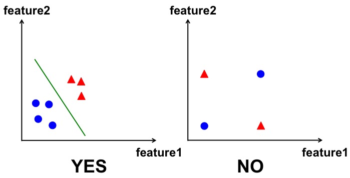
We won't go to many details about the limitation, you can google online for more information. In short, the limitation is that the Perceptron algorithm only works on linearly separable problems. For example, in the following figure, we have two cases. In each case, we have two classes with blue circles, and red triangles. Perceptron can solve the left problem without any problem (you can see the green line can separate the two classes very well). But for the right side, we can see that there's no any single line that can be drawn to separate the two classes, therefore, perceptron algorithm fails to classify them.
You may already guessed that, the solution to the above problem is today's topic - the Multi-Layer Perceptron (MLP), a very popular Artificial Neural Network algorithm that you will use it a lot. It turns out, to solve the above problem, all we need is adding one more layer between the input and output layer. As we talked before, this is the hidden layer, which can actually capture the non-linear relationship in the data, thus can solve the problem by drawing a non-linear boundary to classify the data. Of course, you can add more layers in between, but we will just add one layer for simplicity. (The field of adding more layers to model more combinations of relationships such as this is known as
deep learningbecause of the increasingly deep layers being modeled.)
Let's use the same example we used last time, 4 training data samples, and each has 3 features as shown in the following table.
| Feature1 | Feature2 | Feature3 | Target |
|---|---|---|---|
| 0 | 0 | 1 | 0 |
| 1 | 1 | 1 | 1 |
| 1 | 0 | 1 | 1 |
| 0 | 1 | 1 | 0 |
But this time, we will build a MLP model to solve the same problem, i.e. we will add one hidden layer. In this newly added hidden layer, we have 4 nodes (or we call them neurons, and also, you can use different number of neurons as well). So the structure is like the following figure:
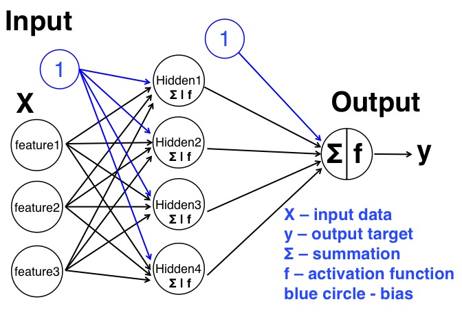
We can see the structure of this Multilayer perceptron is more complicated than the simple perceptron. It has 3 layers, and for the hidden layer, it has 4 nodes/neurons. The summation sign and f in the neurons in the hidden layer indicate that each neuron will work as before: sum all the information from the previous layer, and pass it to a sigmoid activation function. The generated values from these hidden neurons are the outputs for the hidden layer, but they are also the inputs for the output layer. Also, between two different layers, we added the bias term to avoid possible 0 input problem as we described in the previous blog. Overall, there are much more weights in the model, each arrow in the figure is one weight, and we can see that, for each node in one layer, it will connect to all the nodes in the next layer. Therefore, we have much more weights in this MLP.
As most of the important parts of the MLP are similar to the Perceptron model we talked in the previous blog, thus we only talk the difference here.
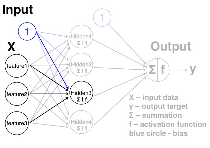
Information propagate forward
As before, the information need propagate forward through the network to the output layer. The difference here is that, each node in the input layer will pass this information to all the nodes in the hidden layer. From the neuron in the hidden layer point of view, each one of them will take all the information all the nodes in the input layer via a set of weights. These weights will be different from other neurons. We can think each neuron connected to the input layers as a simple perceptron we talked before, therefore, all together we will have 4 copies of a parallel perceptron that not interact with each other, as the following figure shows (note that I highlight the part that is essentially a perceptron structure).
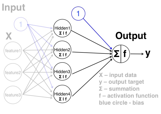
After the neurons get the information from the input layer, they will sum the information, and pass to the sigmoid function to get a value within 0 to 1. Theres 4 numbers that generated from the neurons in the hidden layer will be the input for the output layer. And again, this part is can be thought of the perceptron as the following figure.
learning (backpropagate the error)
The learning of the MLP is more complicated, since now we have three layer with two sets of weights that need to be updated each time from the error. The method that we are going to use is called 'back-propagation', which makes it clear that the errors are sent backwards through the network. The best way to describe back-propagation properly is mathematically. But the purpose of this blog is to show you how they work briefly so that you don't need know exactly the details, as long as you have a general idea how it works. If you want to learn more, check out this blog - a step by step backpropagation example.
Let's look at the code to implement a simple version of MLP, and explain the lines that we didn't cover in the previous blog.
1.  import numpy as np
2.
3.  # define the sigmoid function
4.  def sigmoid(x,deriv=False):
5.      if(deriv==True):
6.          return x*(1-x)
7.      return 1/(1+np.exp(-x))
8.
9.  # define learning rate
10. learning_rate = 0.4
11.
12. # the input data, and we add the bias in line 14
13. X = np.array([[0,0,1],[0,1,1],[1,0,1],[1,1,1]])
14. X = np.concatenate((np.ones((len(X), 1)), X), axis = 1)
15.
16. y = np.array([[0],[1],[1],[0]])
17.
18. np.random.seed(1)
19.
20. # randomly initialize our weights with mean 0 for weights
21. # connect input layer and hidden layer, and connect hidden
22. # layer to output layer
23. weights_0 = 2*np.random.random((4,4)) - 1
24. weights_1 = 2*np.random.random((5,1)) - 1
25.
26. # training the model for 60000 iterations
27. for j in xrange(60000):
28.
29.     # Feed forward through layers 0, 1, and 2
30.     # input layer
31.     layer_0 = X
32.     # layer_1_output is the output from the hidden layer
33.    layer_1_output = sigmoid(np.dot(layer_0,weights_0))
34.     # Note here we add a bias term before we feed them into the output layer
35.     layer_1_output = np.concatenate((np.ones((len(layer_1_output), 1)), layer_1_output), axis = 1)
36.
37.     # layer_2_output is the estimation the model made using current weights
38.     layer_2_output = sigmoid(np.dot(layer_1_output,weights_1))
39.
40.     # how much did we miss the target value?
41.     layer2_error = y - layer_2_output
42.
43.     # let's print out the error we made at each 10000 iteration
44.     if (j% 10000) == 0:
45.         print "Error:" + str(np.mean(np.abs(layer2_error)))
46.
47.     # How much we will change for the weights connect hidden layer
48.     # and output layer
49.     layer2_delta = learning_rate*layer2_error*sigmoid(layer_2_output,deriv=True)
50.
51.     # how much did each hidden node value contribute to the output error (according to the weights)?
52.     layer1_error = layer2_delta.dot(weights_1.T)
53.
54.     # How much we will change for the weights connect the input layer
55.     # and the hidden layer
56.     layer1_delta = learning_rate*layer1_error * sigmoid(layer_1_output,deriv=True)
57.
58.     # update the weights
59.     weights_1 += layer_1_output.T.dot(layer2_delta)
60.     weights_0 += layer_0.T.dot(layer1_delta[:, 1:])
Error:0.4996745482
Error:0.0207575549061
Error:0.0136389203522
Error:0.0108234044104
Error:0.00922321224367
Error:0.00816115693744Explain line by line
You can see most of the lines are very similar to the previous perceptron model, and the only new things is ine line 52.
Line 44: we print the error at n*10000 iterations. And we should see that the error is decreasing, since we update the weights to reduce the error. The more iterations we have, the smaller the error will be. (This is due to the fact that the error we report here is the training error, and it even can be 0 if we over-train the model. We won't talk too much details here, since it is beyond the scope of this blog).
Line 52: uses the
confidence weighted errorfrom output layer to establish an error for hidden layer. To do this, it simply sends the error across the weights from output layer to hidden layer. This gives what you could call a
contribution weighted errorbecause we learn how much each node value in hidden layer
contributedto the error in output layer. We then update the weights that connect the input layer to the hidden layer using the same steps we did in the perceptron implementation.
Visualize ANN
I found this Visualize Neural network very interesting, you can see how the weights and error rates change with training.
Hope you already have a better understanding of the ANN algorithm after reading these blogs, which cover the most important concepts of ANN. Luckily, we don't need to implement ANN by ourselves, since there are already many packages out there for us to use. Next week, we will try to use the implementation of the MLP in sklearn to classify the handwriting digits, while learn more about the Multi-Layer Perceptron that we haven't covered yet.
References and Acknowledgments
A Neural Network in 11 lines of Python (I thank the author, since my blog is modified from his blog).
Machine learning - An Algorithmic Perspective
Single-Layer Neural Networks and Gradient Descent
Machine learning - An Algorithmic Perspective
Single-Layer Neural Networks and Gradient Descent
Subscribe to:
Posts (Atom)