Saturday, October 29, 2016

How to shake a 9-story building on Caltech campus

This week, I am visiting Caltech to do a shaker test, which is a test to shake a 9-story building - The Millikan library, and using sensors to record and measure the response of the building. I am here, because I will put ~30 smartphones on the top of the building, and see if we can use the smartphone to get the fundamental frequency of the building. Also, we will stand on the roof of the building while the shaking, therefore, you will understand that the shaking is not that large, but I was told I can feel the movement of the building for sure. 

How it works

Ok, I know you must curious how they shake the whole building, and whether they are safe or not. Let me explain this to you. 
First, let's see the building from certain distance: 
Figure 1
We know, there are many different things can shake a building, i.e. earthquake, high wind, rain, etc. They all need a force input into the building, for earthquake, the ground movement will introduce a force from the bottom into the building, while for wind, it blows on to the wall of the building, and introduces a lateral force into the building. But for us, how do we introduce a force into the building to shake it? Think about if the building is a toy, and the easiest way is just use your finger to push it on top. But we will not all push the building, instead, we will use something the following device that installed on the top of the building. See the figure below:
You may already have a sense how it works, see the two heavy metal blocks (they call them buckets, which are empty inside, and can be loaded with different configurations of lead weights) in the middle, and they can rotate counter-rotate around the center spindle. When adjust correctly, the shaker can apply a sinusoidal force in any horizontal direction. 
Let me see if I can explain this intuitively. Think about if you rotate a ball with string, you need pull the string with a force to make sure the ball is not moving away. Now think at the same time, you rotate another ball but in the opposite direction, you need pull the two balls with two horizontal forces. And the net effect is the vector sum of the two forces pointing to some direction, we call it resultant force. If we adjust the rotation rate of the rotating two balls, we will have the resultant force pointing to the same direction, but the force will change from large to small, and then from small to large in the exactly opposite direction (180 degree), the so called sinusoidal force. 
Figure 3
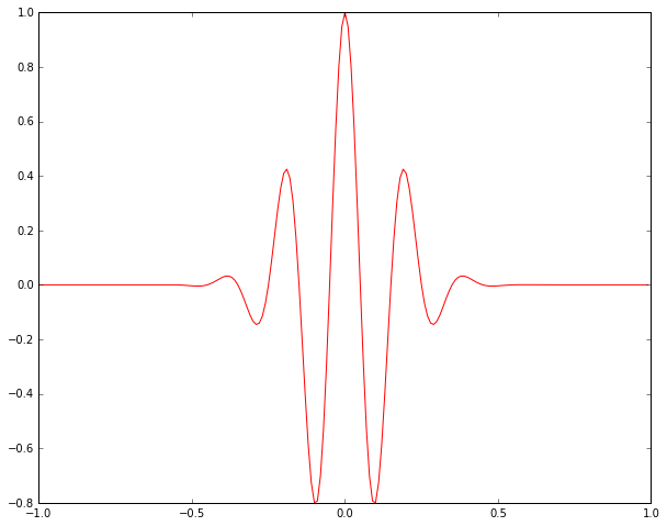
The following figure shows the time changing of the amplitude of the resultant force. 
Figure 4
We know that, building has its own natural frequency (it is one of the most important properties of the building), which will oscillate when apply a force, and it will have much larger movement when the frequency of the applied force is similar to the natural frequency. See the following animation, when moving with different frequencies, the movement of the different color ball is different (the length of the stick defines the natural frequency).
Figure 5
Therefore, if we adjust the sinusoidal force with the frequency similar to the natural frequency of the building, the building will start to vibrate. But don't worry, the maximum of the shaking is about 1 mm on the top of the building, which means, a lot of people actually may not feel the movement of the building. 

Of course, this shaker can also apply a twist on the building, just adjust the rotation of the two blocks, but this is beyond the simple explaination of this blog, see more information in the references. 

The purpose of the test

The purpose of the test is to identify the natural frequency of the building in different directions, therefore, you can keep a time history of the changes of it. It can be a health state indicator of the building, for example, if after an earthquake, there're some damages to the building, you will see a large change of the natural frequency. See the details in the references. 

Acknowledgement

We thank Professor Monica Kohler, Professor Thomas HeatonLucy Yin, and Anthony Massari for the opportunity and help with the tests. Figures except the shaker are all from online resources, I thank the authors as well.

References

Saturday, October 22, 2016

Signal Processing: Cross-correlation in the frequency domain

Cross-corrlation is a technique widely used in many fields. I won't go to the details of it, since wikipedia already gave a very nice introduction. In seismology, cross correlation is a great tool, for example, to find the amount of shift of one signal recorded different locations on earth, you can use cross correlation; using ambient noise cross correlation, we can find the empirical green's function between two seismic stations; to monitor the nuclear tests around the world, cross correlation also be used to do the pattern recognition on the waveforms recorded. Of course, there are still many other use cases in seismology, therefore, today we will talk about how to do cross correlation in frequency domain. You can find all the scripts at Qingkai's Github
You can also do the cross correlation in time domain. But doing this in frequency domain is very simple, and clear, and of course faster as well (I tested both version in the frequency/time domain). 
import numpy as np
from obspy.core import read
import matplotlib.pyplot as plt
from numpy.fft import fft, ifft, fftshift
%matplotlib inline

Let's create the first signal

For simplicity, we will create the first signal using scipy. We will create a gaussian pulse. 
from scipy import signal
t1 = np.linspace(-1, 1, 2 * 100, endpoint=False)
sig1 = signal.gausspulse(t1, fc=5)
plt.figure(figsize=(10,8))
plt.plot(t1, sig1, 'r')
plt.show()

Create the 2nd signal by simply shift it

For simplicity, we will just shift the first signal by 50 data points, and use it as the second signal. We will use the function we created in the previous post - shift signal in frequency domain to shift the signal in the frequency domain. 
def nextpow2(i):
    '''
    Find the next power 2 number for FFT
    '''

    n = 1
    while n < i: n *= 2
    return n

def shift_signal_in_frequency_domain(datin, shift):
    '''
    This is function to shift a signal in frequency domain. 
    The idea is in the frequency domain, 
    we just multiply the signal with the phase shift. 
    '''
    Nin = len(datin) 

    # get the next power 2 number for fft
    N = nextpow2(Nin +np.max(np.abs(shift)))

    # do the fft
    fdatin = np.fft.fft(datin, N)

    # get the phase shift, shift here is D in the above explanation
    ik = np.array([2j*np.pi*k for k in xrange(0, N)]) / N 
    fshift = np.exp(-ik*shift)

    # multiple the signal with shift and transform it back to time domain
    datout = np.real(np.fft.ifft(fshift * fdatin))

    # only get the data have the same length as the input signal
    datout = datout[0:Nin]

    return datout
# This is the amount we will move
nShift = 50

# generate the 2nd signal
sig2 = shift_signal_in_frequency_domain(sig1, nShift)

# plot two signals together
plt.figure(figsize=(10,8))
plt.plot(sig1, 'r', label = 'signal 1')
plt.plot(sig2, 'b', label = 'signal 2')
plt.legend()
plt.show()

Frequency domain cross correlation

Shift a signal in the frequency domain is quite simple. 
  1. zero-pad the input signals or apply a taper as we talked last week. (I didn't do this, since I know my two signal is zero at both ends, so I skip it)
  2. take the FFT of both signals
  3. multiply the first signal, and the reverse of the signal (or the conjugate, note that in the frequency domain, the complex conjugation is equivalent to time reversal in the time domain)
  4. do the inverse FFT and get the shift
reference:
stackexchange
def cross_correlation_using_fft(x, y):
    f1 = fft(x)
    
    # flip the signal of y
    f2 = fft(np.flipud(y))
    cc = np.real(ifft(f1 * f2))

    return fftshift(cc)
 
# shift &lt; 0 means that y starts 'shift' time steps before x 
# shift &gt; 0 means that y starts 'shift' time steps after x
def compute_shift(x, y):
    # we make sure the length of the two signals are the same
    assert len(x) == len(y)
    c = cross_correlation_using_fft(x, y)
    assert len(c) == len(x)
    zero_index = int(len(x) / 2) - 1
    shift = zero_index - np.argmax(c)
    return shift
calculate_shift = compute_shift(sig1, sig2)
print('The shift we get from cross correlation is %d, the true shift should be 50'%calculate_shift)
You can see the result will be 50, which is our correct shift. 

Saturday, October 15, 2016

Signal Processing: Why do we need taper in FFT

When we try to study the frequency content of a signal, FFT is always the tool we use. Also, a lot of times, you hear others talking about 'we applied a XX taper before we conduct the FFT'. Why we need a taper before FFT? This week, we will talk about what is a taper, and why we need it. You can find all the script at Qingkai's Github. Let's first look at an example below:
In [1]:
import numpy as np
from scipy import fft, arange
import matplotlib.pyplot as plt
from scipy import signal
%matplotlib inline
plt.style.use('seaborn-poster')
In [2]:
def plotSpectrum(t, y,Fs):
    """
    Function to plot the time domain and frequency domain signal
    """
    n = len(y) # length of the signal
    k = arange(n)
    T = n/Fs
    frq = k/T # two sides frequency range
    frq = frq[range(n/2)] # one side frequency range

    Y = fft(y)/n # fft computing and normalization
    Y = Y[range(n/2)]    
    
    # plot time domain and frequency domain signal
    plt.subplot(2,1,1)
    plt.plot(t,y)
    plt.xlabel('Time')
    plt.ylabel('Amplitude')
    plt.subplot(2,1,2)
    plt.stem(frq,abs(Y),'r')
    plt.xlabel('Freq (Hz)')
    plt.ylabel('|Y(freq)|')
    plt.tight_layout()
    plt.show()

Example 1 (5 Hz sine wave)

Let's create a 5 Hz sine signal with a sampling rate 100 Hz (this is saying within 1 second, we have 100 data points to represent this sine signal). We can see the time domain signal in the following top figure with 5 cycles within 1 second. The bottom figure shows the FFT spectrum amplitude, and we see a very clear 5 Hz signal. So far so good, and it all looks normal.
In [3]:
Fs = 100.0  # sampling rate
Ts = 1.0/Fs # sampling interval
t = arange(0,1,Ts) # time vector
ff = 5;   # frequency of the signal
# create the signal
y = np.sin(2*np.pi*ff*t + 5)

plotSpectrum(t, y,Fs)

Example 2 (same 5 Hz sine wave, but a little shoter)

Using the same signal as the above, we just shrink the signal from 1 sec to 0.5 sec, as the top figure shows. But when we look at the FFT spectrum, somehow we are not getting the clear 5 Hz signal anymore. Instead, we have a large peak at 5 Hz, but also small peaks at other frequencies. What happened? We are pretty sure that the signal is a 5 Hz signal, where other frequency content comes from?
In [4]:
# let's extend the signal from 1s to 0.5s
t = arange(0,0.5,Ts)

# make sure we are still using 5 Hz as the frequency of the signal
ff = 5;
y = np.sin(2*np.pi*ff*t + 5)
plotSpectrum(t, y,Fs)

Why this happens

Well, if we look at the first example and second example more carefully, we will notice the difference: the start and end point of the signal in example 1 are all -1. But in the second example, the start point is -1, and the end point is 1. Is this the cause of the problem? Yes! When we conduct FFT on a finite length signal, we actually assume the signal repeat itself to a infinite length signal and connecting the end point with the start point (you can also think the signal is has a period of whole length). But in the second example, when we connect the signal, there is a discontinuity as the following figure shows. This kind of discontinuity in the signal usually introduces other frequency signals, and smear the true spectrum by spreading the peak to the surrounding frequencies. It is like the energy leak to other frequencies, so people call it spectrum leakage.

How can we reduce the leakage

This is where the taper or window function comes in. We can multiply a smooth window function to make the connecting points smoother, usually this window function is also called taper. A typical taper usually has a gradual decreasing of amplitude to zero towards the edge. For example, if we plot a cosine taper in the time and frequency domain, it will look like the following figure.

Cosine taper

In [5]:
n = len(t) # number of points
window = signal.cosine(n)
plotSpectrum(t, window,Fs)

Apply the taper

This windowing process consists of multiplying the time record by a finite-length window with an amplitude that varies smoothly and gradually toward zero at the edges. Let's apply the cosine taper to the signal, and we can see the signal now has 0 at both the start and end point. The FFT spectrum has less leakage than before.
In [6]:
# apply the taper to the signal
y_tapered = window * y 
plotSpectrum(t, y_tapered,Fs)

Try different window

There are many different types of window function, how to choose them depends on your need or your problem at hand. In the following, I will plot some common window functions, you can get a sense of what they look like.

Blackman

In [7]:
window = signal.blackman(n)
plotSpectrum(t, window,Fs)

y_tapered = window * y 
plotSpectrum(t, y_tapered,Fs)

Hanning

In [8]:
window = signal.hanning(n)
plotSpectrum(t, window,Fs)

y_tapered = window * y 
plotSpectrum(t, y_tapered,Fs)

flattop

In [9]:
window = signal.flattop(n)
plotSpectrum(t, window,Fs)

y_tapered = window * y 
plotSpectrum(t, y_tapered,Fs)

Tukey

In [10]:
window = signal.tukey(n)
plotSpectrum(t, window,Fs)

y_tapered = window * y 
plotSpectrum(t, y_tapered,Fs)

Parzen

In [11]:
window = signal.parzen(n)
plotSpectrum(t, window,Fs)

y_tapered = window * y 
plotSpectrum(t, y_tapered,Fs)