I am now reading
Data analysis a bayesian tutorial, in chapter2, the single parameter estimation, it starts with a simple coin-tossing example to illustrate the idea of Bayesian analysis. I am going to use python to reproduce the figure in this example. I won't go into the details of this example, but will just describe it in a brief manner. You can always check out the book of this example (it is a nice example!). Here I will just show the python script I wrote to do the simulation, and generate a figure like the one used on page 16 in the book.
Brief description of the example: is this a fair coin?
If you toss a coin N times, and got H times heads and T times tails, how do you know if this is a fair coin or a bias coin? How certain you are about your conclusion?
We use Bayesian analysis to answer this question, which formulated as follows:
\(\begin{equation}
prob(H|\{data\},I)\propto prob(\{data\}|H,I)\times prob(H|I)
\end{equation}\)
The left hand is posterior, that is, the probability of the parameter H given the data we observed and the background information we already known. H is the probability of getting heads. The right hand are the likelihood and prior individually. The likelihood is a measure of the chance that we would have obtained the data that we actually observed, if the value of the H was given. The prior represents what we know about the coin given only the information I. Because we don't have an idea of the fairness of the coin, we just set the prior to be a uniform distribution. And if we assume that the flips of the coin were independent events, so that the outcome of one did not influence that of another, then the likelihood probability can be modeled by using a binomial distribution. The likelihood function is showing below, and R is the number of cases that we got heads.
\(\begin{equation}
prob(\{data\}|H,I)\propto {{H}^{R}}{{(1-H)}^{N-R}}
\end{equation}\)
Therefore, if we do the tossing multiple times, and plot the posterior vs the parameter we want to estimate, H. Then we can see the following figures as the results. The total number of tosses in each figure is 0, 1, 2, 3, 4, 8, 16, 32, 64, 128, 256, 512, 1024, 2048, 4096 times.
This figure is easy to interpret, the x-axis is the parameter we want to estimate H, that is the probability of getting heads. And the y-axis shows us the posterior probability. What we want to see is a narrow peak at a certain value of x, that is our best estimation, and the width of the peak represents the uncertainty of our estimation. Two extreme values are H = 0, and H = 1. If H = 0, this means that the probability of getting head is 0, that is the coin has two tails in both sides. H = 1 is the opposite way, that we have two heads at both sides. The value between 0 and 1 is telling us the fairness of the coin. We can see from the following evolution as the number of tosses increase. When N = 0, because there's no data, so it is 1 everywhere, this means that we have no idea which x is the best estimation, so they have a equal weight. Then when N = 1, we get a head, we can see that we have a line goes for H = 0 and rises linearly to having the largest value at H =1. Although H = 1 is our best estimate, the posterior pdf indicates that this value is not much more probable than many others. The only thing we can say is that the coin is not double-tailed. When N = 2, we get another head, the posterior pdf becomes slightly more peaked towards H = 1. N = 3, we observe a first tail, this drag the posterior to the H = 0 side, now we can see the pdf at H = 1 drops to 0, saying that double-headed is not possible. And when more and more observations available, we starting to see the posterior pdf becomes narrower and narrower and peaked at 0.25. This means that we are more and more confident in our estimation.
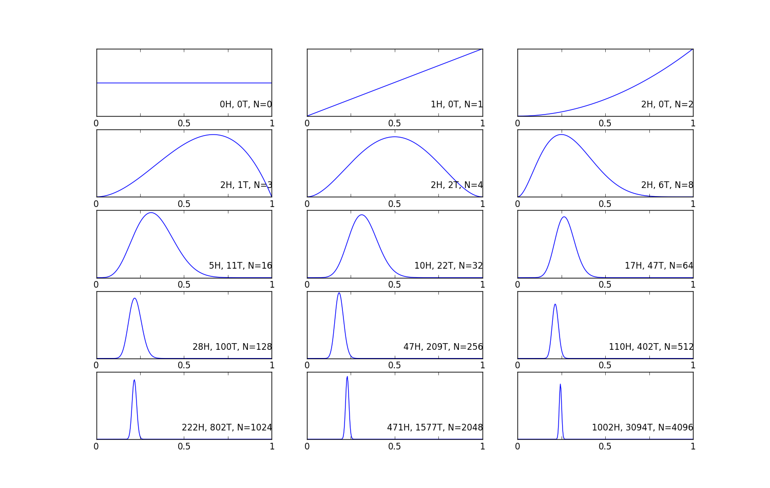
These figures show the evolution of the posterior pdf for the probability of getting heads of a coin on x-axis, and prob(H|{data}, I) on y-axis, as the number of data available increases. The 3 numbers on the right bottom is number of heads, number of tails, and total number of the tosses.
This example illustrate the basics of the Bayesian analysis, and from here, what you want to do is based on the data we observed, we want to find the best H value that maximize the posterior pdf, this is actually the idea of MAP.
In the next post, we will try two alternate prior, and see how they will affect the result.
You can download the python script from my github:
Qingkai's github
